A Causal Impact Study of The Queen’s Gambit on Chess
Analyzing the “Anya Taylor-Joy Effect”
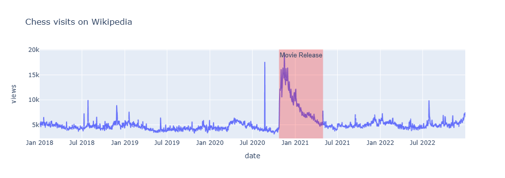
The release of The Queen’s Gambit on Netflix in October 2020 coincided with a massive global spike in chess interest. I would like to explore if there has been any relevant effect that is measurable and attributed to the Netflix show. Was this just a continuation of the “pandemic hobby” trend, or did Beth Harmon truly change the game?
In this post, I’ll describe causal inference toy analysis hosted in my queens_gambit_causal_impact repository, which attempts to isolate the “Netflix effect” from any other change that may have influenced.
0. Summary
This analysis quantifies the specific impact of the Netflix miniseries The Queen’s Gambit on the popularity of chess. I’ll use Bayesian structural time-series models, moving beyond simple line charts to estimate a counterfactual: What would chess interest have looked like in late 2020 if the show had never been released? Using Wiki page visits, the analysis provides a statistical smoking gun for the show’s influence.
1 Why Causal Impact?
Traditional metrics often fail when multiple variables shift at once. In late 2020, we had two massive drivers for chess: the ongoing COVID-19 lockdowns and the release of the show.
We use the CausalImpact methodology because it is autoregressive and simple to use when we have limited data. By picking variables that are correlated with our target (chess) but unaffected by the “treatment” (the show), such as general interest in other board games, we can predict the baseline trend. The difference between this predicted baseline and the actual observed data is the “causal impact”.
2 The Queen’s Gambit Phenomenon
When The Queen’s Gambit premiered on October 23, 2020, it became a cultural juggernaut. However, chess was already growing in early 2020 due to the pandemic. The challenge of this analysis is to separate these two waves. As noted in the project, the “treatment” is defined precisely as the show’s release date, allowing us to see if the slope of interest changed significantly enough to be considered a direct result of the series.
3 Methodology
3.1 Data Acquisition
The study pulled daily Wikipedia pageviews for games like Chess, Backgammon, and other hobbies/games. We’ll use these for our estimation. This initial exploration was crucial because it confirmed that a simple “before vs. after” comparison would be flawed; we had to account for the fact that chess was already trending upward due to global lockdowns before the show even premiered.
| date | Backgammon | Chess | Gardening | Guitar | Origami | Painting | Piano | Rubik’s Cube | Sudoku | Yoga |
|---|---|---|---|---|---|---|---|---|---|---|
| 2018-01-01 | 3239 | 4906 | 485 | 2309 | 1031 | 1480 | 1941 | 2361 | 1803 | 3986 |
| 2018-01-02 | 2480 | 5270 | 568 | 2405 | 1087 | 2154 | 2335 | 2303 | 2097 | 4981 |
| 2018-01-03 | 2228 | 5040 | 540 | 2504 | 1265 | 2057 | 2295 | 2322 | 1971 | 4867 |
| 2018-01-04 | 2181 | 5346 | 569 | 2575 | 1142 | 2149 | 2149 | 2337 | 1791 | 4932 |
| 2018-01-05 | 2153 | 5599 | 501 | 2343 | 1202 | 2159 | 2177 | 2346 | 1922 | 4520 |
3.2 Stationarity and Pre-processing
Before modeling, it is essential to examine the properties of the time series. In the notebook, I looked at the trends to ensure we weren’t being misled by seasonal noise or erratic outliers. While the Causal Impact package (based on BSTS) handles non-stationary data better than traditional OLS regressions, checking for stationarity and understanding the underlying growth components helps in selecting the correct “pre-intervention” period. This ensured the model was trained on a stable relationship between the target and the predictors.
3.3 Synthetic Control creation
To isolate the “Netflix effect”, I constructed a Synthetic Control. This involved selecting the suite mentioned in 3.1. I fitted a Linear Regression on the other “hobbies” by predicting Chess. The logic here, as commented in the code, is that these terms share the same “lockdown DNA” as chess but have no reason to spike because of a TV show about a Grandmaster. By combining these variables, the model creates a “Synthetic Chess” by taking the games that were mostly showing more correlation with chess.
| date | Backgammon | Chess | Gardening | Guitar | Origami | Painting | Piano | Rubik’s Cube | Sudoku | Yoga | Chess_synthetic |
|---|---|---|---|---|---|---|---|---|---|---|---|
| 2018-01-01 | 3239 | 4906 | 485 | 2309 | 1031 | 1480 | 1941 | 2361 | 1803 | 3986 | 6087.935964 |
| 2018-01-02 | 2480 | 5270 | 568 | 2405 | 1087 | 2154 | 2335 | 2303 | 2097 | 4981 | 5544.680612 |
| 2018-01-03 | 2228 | 5040 | 540 | 2504 | 1265 | 2057 | 2295 | 2322 | 1971 | 4867 | 5273.755123 |
| 2018-01-04 | 2181 | 5346 | 569 | 2575 | 1142 | 2149 | 2149 | 2337 | 1791 | 4932 | 5048.938634 |
| 2018-01-05 | 2153 | 5599 | 501 | 2343 | 1202 | 2159 | 2177 | 2346 | 1922 | 4520 | 5057.021750 |
3.4 Causal Impact
With the data prepared, I applied the CausalImpact algorithm. This technique uses a Bayesian structural time-series model to predict the counterfactual. Instead of a simple linear projection, the model uses the behavior of the synthetic control (the other board games) to estimate what the chess trend should have looked like post-October 2020.
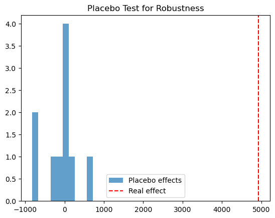
3.5 Placebo Tests
The model then predicted what chess interest should have been how chess and the other board games were performing before the release date. I performed a total of 10 placebo tests by picking random dates before the show and saw the results.
4 Findings
By looking at the exploratory time series, it looks that chess page visits spiked from averaging 4.5k in May-Oct 2020 to 9k in Nov-Apr 2020-21, after the movie release. From the picture below, you can immediately notice that it looks there’s been an impact, right?
But is this 102% lift really causal? If yes, how much?
I applied the Causal Impact function and you can see the result below:

With the function impact.summary(‘report’), you can read the explanation provided directly by the library.
During the post-intervention period, the response variable had an average value of approx. 8990.02. By contrast, in the absence of an intervention, we would have expected an average response of 4059.16. The 95% interval of this counterfactual prediction is [3154.04, 4968.13]. Subtracting this prediction from the observed response yields an estimate of the causal effect the intervention had on the response variable. This effect is 4930.86 with a 95% interval of [4021.89, 5835.98].
The above results are given in terms of absolute numbers. In relative terms, the response variable showed an increase of +121.48%. The 95% interval of this percentage is [99.08%, 143.77%].
This means that the positive effect observed during the intervention period is statistically significant and unlikely to be due to random fluctuations. It should be noted, however, that the question of whether this increase also bears substantive significance can only be answered by comparing the absolute effect (4930.86) to the original goal of the underlying intervention.
The probability of obtaining this effect by chance is very small (Bayesian one-sided tail-area probability p = 0.0). This means the causal effect can be considered statistically significant.
5 The importance of Placebo tests
To validate these findings, I used Placebo Tests (or “A/A testing” in a temporal sense). I ran the same model 10 times on a date before the show was released—where we know no treatment occurred—we can check if the model incorrectly finds an effect.
As highlighted in the project’s logic, if the model shows a “causal impact” on a random date in July 2020, our model is likely picking up noise. Because the placebo tests in this study showed no significant impact, we can have much higher confidence that the October spike was truly caused by the show. See picture below, the red line is the result given by our model and the blue bars are the placebo test results:
Sources:
Kay H. Brodersen, Fabian Gallusser, Jim Koehler, Nicolas Remy, Steven L. Scott - Inferring causal impact using Bayesian structural time-series models - 2015
Matheus Facure - Causal Inference in Python - 2023